This is the third in a series of posts that seek to recreate the methods used in Future ozone-related acute excess mortality under climate and population change scenarios in China: A modeling study. All the posts build on my previous post on forecasting, by using data available from national and international research initatives to project future scenarios for complex systems including atmospheric chemistry, population dynamics, and mortality. This post focuses on the third projection: mortality rate.
The previous two posts discussed projecting future ozone concentrations using global climate models and projecting population dynamics to understand the size and age structure of future demographic scenarios. This post will describe methods for projecting national mortality rates to adjust epidemiological mortality counts collected at the city level. In the next post, the three preceding projections will be brought together to estimate the future excess mortality attributable to ozone concentration change.
Methods: Projecting National Mortality Rates for City-Level Adjustments
Overview of Analysis
The workflow for this analysis involves recreating the methods used in the PLOS Medicine article.
"City-level baseline cause-specific, age-group-specific, and seasonal mortality counts were also obtained from the previous publication [46]. Future changes in age-group-specific mortality rates and their 95% probability intervals (PIs) in 2050–2055 versus 2010–2015 were obtained using data from the United Nation’s 2017 World Population Prospects [49] and the MortCast package, which projects age-specific mortality rates using the Kannisto, Lee–Carter, and related methods as described in Ševčíková et al. [50].
The calculated changing ratios of mortality rates in 2050–2055 versus 2010–2015 in China were 0.68 (95% PI: 0.35–1.02) for individuals aged 5–64 years, 0.50 (95% PI: 0.26–0.73) for individuals aged 65–74 years, and 0.83 (95% PI: 0.61–1.05) for individuals aged ≥75 years. Because no projection data for city-level cause-specific and seasonal mortality rates were available in China, we assumed constant daily mortality counts for each city in the future when estimating future cause-specific and seasonal ozone-related acute excess mortality."
To break down this excerpt into discrete steps:
- load the appropriate packages
- Use life expectancies and mathematical parameters to estimate mortality rates
- Aggregate mortality rates into age brackets (5-64, 65-74, ≥75)
- Calculate mortality rate changing ratios to adjust mortality counts for future scenarios
Analysis
As the excerpt notes, the MortCast package provides the data and algorithms for projecting life expectancies and mortality rates. The package vignette provides an easy step-by-step process for projecting life expectancies and mortality rates.
MortCast loads the wpp2017 package as a dependency, meaning the wpp2017 package will load whenever MortCast is loaded, and the data available in wpp2017 will be available for analysis. wpp2017 is the 2017 revision of the World Population Prospects available from the United Nations Population Division. The datasets historical and future mortality rates for men and women (mxM and mxF, respectively), historic life expectancies with one entry per country (e0M an e0F), and projected life expectancies (e0Mproj and e0Fproj). The projected data also includes lower and upper 80 and 95% confidence values denoted by a number, 80 or 95, and a letter, u or l (i.e. e0Fproj80l for the lower 80% confidence interval).
A quick look at the mxM dataset shows that each row denotes a separate age group within a given geographic area, either a country, region, or globally. The following columns indicate the mortality rates from 1950 through 2095 in five-year increments.
library(MortCast)
library(tidyverse)

data(mxM, mxF, e0F, e0M, e0Fproj, e0Mproj, package = "wpp2017")

head(mxM)[,1:6]
## country_code age name 1950-1955 1955-1960 1960-1965
## 1 900 0 WORLD 0.165328131 0.150482547 0.139673526
## 2 900 1 WORLD 0.021953698 0.019297510 0.017989641
## 3 900 5 WORLD 0.006525011 0.005604632 0.005010102
## 4 900 10 WORLD 0.003927849 0.003301526 0.003042159
## 5 900 15 WORLD 0.004791867 0.004196964 0.003711798
## 6 900 20 WORLD 0.005960807 0.005232142 0.004545673The mortality rate datasets can be subset for a specific country (“United States of America”), and then extrapolated into higher age brackets using the Coherent Kannisto method.
country <- "United States of America"
mxm <- subset(mxM, name == country)[,4:16] %>%
  slice(-2)
mxf <- subset(mxF, name == country)[,4:16] %>%
  slice(-2)
rownames(mxm) <- rownames(mxf) <- c(0, seq(5, 100, by=5))
# Step 1: extrapolate from 100+ to 130+ using Coherent Kannisto
mx.cokannisto <- cokannisto(mxm, mxf, proj.ages = seq(100, 130, by = 5))The projected mortality rates serve as the input for estimating the Coherent Lee-Carter parameters.
# Steps 2-5: estimate coherent Lee-Carter parameters
lc.est <- lileecarter.estimate(mx.cokannisto$male, mx.cokannisto$female,
                               ax.index = ncol(mx.cokannisto$male), ax.smooth = TRUE)
The projected mortality rates and Lee-Carter parameters then serve to predict future mortality rates.
# Steps 6-9: project future mortality rates based on future
# life expectancies from WPP2017

# add 2010-2015 from E0F and E0M to the projections, which start with 2015-2020
e0f <- as.numeric(cbind(subset(e0F, name == country)[,ncol(e0F)], subset(e0Fproj, name == country)[-(1:2)]))
e0m <- as.numeric(cbind(subset(e0M, name == country)[,ncol(e0M)], subset(e0Mproj, name == country)[-(1:2)]))
names(e0f) <- names(e0m) <- c("2010-2015", colnames(e0Fproj)[-(1:2)])

# output: predict age-specific mortality rates
# input: future life expectancies for male and female (e0m and e0f) projected using CR Lee-Carter parameters
pred <- mortcast(e0m, e0f, lc.est)

pred$female$mx[,1:8]
## 2010-2015 2015-2020 2020-2025 2025-2030 2030-2035
## 0 1.727865e-03 1.454915e-03 1.243351e-03 1.081951e-03 9.504432e-04
## 5 1.872370e-04 1.794287e-04 1.699460e-04 1.582135e-04 1.465218e-04
## 10 5.174517e-05 4.549989e-05 4.024617e-05 3.582261e-05 3.203014e-05
## 15 7.145375e-05 6.103565e-05 5.275868e-05 4.625510e-05 4.087172e-05
## 20 2.142758e-04 1.960232e-04 1.789339e-04 1.625921e-04 1.477484e-04
## 25 4.304136e-04 4.115805e-04 3.891644e-04 3.618923e-04 3.348557e-04
## 30 5.636836e-04 5.375073e-04 5.070990e-04 4.708712e-04 4.351934e-04
## 35 6.925988e-04 6.495049e-04 6.046831e-04 5.566140e-04 5.109450e-04
## 40 9.506549e-04 8.816279e-04 8.135491e-04 7.445344e-04 6.803447e-04
## 45 1.457305e-03 1.349826e-03 1.244374e-03 1.138080e-03 1.039438e-03
## 50 2.204266e-03 2.039974e-03 1.879343e-03 1.718052e-03 1.568600e-03
## 55 3.176847e-03 2.934189e-03 2.698850e-03 2.464652e-03 2.248416e-03
## 60 4.347429e-03 3.978109e-03 3.632026e-03 3.300754e-03 2.999724e-03
## 65 6.473885e-03 5.910431e-03 5.386472e-03 4.889359e-03 4.439313e-03
## 70 1.025731e-02 9.368684e-03 8.541980e-03 7.757275e-03 7.046534e-03
## 75 1.758108e-02 1.615121e-02 1.481319e-02 1.353546e-02 1.237102e-02
## 80 3.250012e-02 3.016524e-02 2.795754e-02 2.582666e-02 2.386344e-02
## 85 6.481210e-02 6.115268e-02 5.763470e-02 5.418056e-02 5.094214e-02
## 90 1.323046e-01 1.276102e-01 1.229959e-01 1.183604e-01 1.139118e-01
## 95 2.488257e-01 2.449055e-01 2.409727e-01 2.369377e-01 2.329811e-01
## 100 4.078917e-01 4.068321e-01 4.057547e-01 4.046339e-01 4.035193e-01
## 105 5.634965e-01 5.627641e-01 5.620185e-01 5.612417e-01 5.604682e-01
## 110 7.085975e-01 7.081369e-01 7.076676e-01 7.071784e-01 7.066909e-01
## 115 8.217117e-01 8.214446e-01 8.211724e-01 8.208885e-01 8.206055e-01
## 120 8.971328e-01 8.969870e-01 8.968383e-01 8.966833e-01 8.965287e-01
## 125 9.427325e-01 9.426559e-01 9.425778e-01 9.424963e-01 9.424151e-01
## 130 9.728245e-01 9.727850e-01 9.727447e-01 9.727027e-01 9.726607e-01
## 2035-2040 2040-2045 2045-2050
## 0 8.429618e-04 7.473769e-04 6.611234e-04
## 5 1.349762e-04 1.234396e-04 1.121889e-04
## 10 2.877118e-05 2.577503e-05 2.300796e-05
## 15 3.640256e-05 3.238600e-05 2.873451e-05
## 20 1.342653e-04 1.214303e-04 1.092958e-04
## 25 3.082758e-04 2.817821e-04 2.559847e-04
## 30 4.003191e-04 3.656688e-04 3.319963e-04
## 35 4.677056e-04 4.255167e-04 3.849865e-04
## 40 6.207383e-04 5.632391e-04 5.084044e-04
## 45 9.480277e-04 8.599575e-04 7.760356e-04
## 50 1.430300e-03 1.297165e-03 1.170370e-03
## 55 2.048976e-03 1.857363e-03 1.675108e-03
## 60 2.726180e-03 2.465722e-03 2.219439e-03
## 65 4.031797e-03 3.644608e-03 3.279012e-03
## 70 6.402661e-03 5.790612e-03 5.212407e-03
## 75 1.130966e-02 1.029441e-02 9.328979e-03
## 80 2.205440e-02 2.030461e-02 1.862119e-02
## 85 4.790567e-02 4.491593e-02 4.198548e-02
## 90 1.096422e-01 1.053371e-01 1.010108e-01
## 95 2.291016e-01 2.251030e-01 2.209913e-01
## 100 4.024110e-01 4.012520e-01 4.000422e-01
## 105 5.596979e-01 5.588914e-01 5.580482e-01
## 110 7.062051e-01 7.056961e-01 7.051636e-01
## 115 8.203234e-01 8.200277e-01 8.197183e-01
## 120 8.963746e-01 8.962130e-01 8.960439e-01
## 125 9.423340e-01 9.422491e-01 9.421602e-01
## 130 9.726189e-01 9.725751e-01 9.725292e-01We see that the mortality rates in China are all greatly reduced between 2015-2095 (bear in mind that the plot uses a log scale to allow all the age groups to be plotted concurrently).
pred.plot.data <-
pred$female$mx %>%
  cbind(age_group = row.names(.)) %>%
  as_tibble() %>%
  gather(key = year, value = mort.rate, -age_group) %>%
  mutate(year = as.numeric(stringr::str_replace(year, "-.*", ""))) %>%
  mutate(mort.rate = round(as.numeric(mort.rate), 5),
         age_group = as.numeric(age_group))


library(directlabels)

pred.plot.data %>%
  ggplot(., aes(x = year, y = mort.rate, group = age_group, color = age_group)) +
  theme(legend.title = element_text("Age Group"))+
  labs(title = "Projected Mortality Rates (2015-2095)",
       y = "Mortality Rate")+
  scale_color_gradient(low = "red", high = "blue")+
  scale_y_log10()+
  geom_line()  +
  geom_dl(aes(label = age_group), method = list(dl.combine("last.points"), cex = 0.8)) +
  guides(color=FALSE)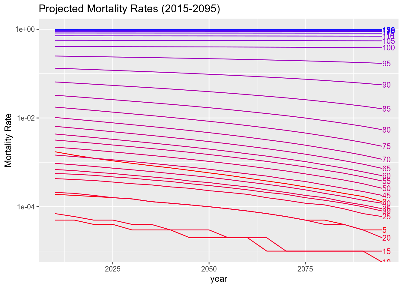
The ultimate purposes of the projected mortality rates is to determine the ratio of future to present mortality rates within age groups in 2050-2055 versus 2010-2015. I have attempted to reproduce these results in many ways: using the wpp2017 data by itself, weighting the projected mortality rates by the population projections under the five shared socioeconomic projections, and through age-group standardization relative to a single population projection scenario. Unfortunately, I have been unable to produce the results exactly. I suspect that the issues arise either becaue the article uses mortality rates that are directly related to the Chinese mortality counts (this data is unavailable publicly) or the exact weighting or projections are not clear.
Update: The co-authors were willing to share the code snippet with me and I have reproduced the article’s mortality rate ratios. The co-authors used the upper and lower 95% confidence interval datasets in the wpp2017 package to produce the median values and also aggregate the age bands using the accompanying population projection datasets. Because I did not produce the analysis, I will not share the code, however I am sure the co-authors would be willing to share it with other enthusiasts.